4. Illustration: exploring an apple tree orchard

Todo

This section has to be validated (e.g., translate aml code into python)

Let us now illustrate the usage of openalea.mtg package together with other packages such as openalea.sequence_analysis in a real application. To do this, we shall consider an apple tree orchard and show how a plant architecture database can be created from observations [24]. Then, we shall use this database to illustrate the use of specific tools employed to explore plant architecture databases.

4.1. Biological context and data collection

The application is part of a general selection program, conducted at INRA (Institut National de la Recherche Agronomique), and aims to improve apple tree species as regards morphological characters and more classical criteria such as fruit quality and disease resistance. In this particular example, two apple tree clones were chosen for their contrasting growth and branching habits. The first clone (‘Wijcik’) exhibits a very particular growth and branching habit, characterised by short internodes, great diameters and the absence of long axillary branches. By contrast, the second clone (‘Baujade’) exhibits many long and flexible branches. A population of 102 hybrids was obtained by crossing these two clones. The objective of this work was to study how morphological characters, such as the length of the internodes or the number of long lateral branches, are distributed within the progeny.

Creation of the database: The branching systems borne by the three-year-old annual shoot of the trunk is described for each individual. The branching system is first broken down into axes i.e. linear portions of stem derived from the same bud. Each axis is then divided into portions created during the same year (called annual shoots). When cessation and resumption of growth occur within a year, the annual shoot can be split into growth units, i.e. portions created over the same period (or between two resting periods). Finally, the growth units can be divided into internodes, i.e. portions of stem between two leaves. Regarding these successive decompositions, a given branching system is simultaneously considered at four scales. The different plant components and their connections are represented into a code file as explained previously.

In order to give a quantitative idea of the total resources necessary for an application of this size, it should be noted that all the measures were carried out by a team of 6 persons over 5 days. The collected data, initially recorded on paper, were then computer-entered by 1 person over 20 days using a text editor and consists of a file of approximately 16000 lines of code. The corresponding MTG is constructed in 45 seconds on a SGI-INDY workstation. It contains about 65000 components and some 15000 attributes. The overall size of the database is 7 Mb.

4.2. 3D visualisation of real plants

To build the database associated with the collected data, the AMAPmod system is launched and an MTG is built from the encoded plant file:

plant_database = MTG("wij.mtg")

The primitive MTG attempts to build a formal representation of the orchard, checking for syntactic and semantic correctness of the code file. If the file is not consistent, the procedure outputs a set of errors which must be corrected before applying a new syntactic analysis. Once the file is syntactically consistent, the MTG is built and is available in the variable plant_database. However, for efficiency reasons, the latest constructed MTG is said to be ‘’active’’: it will be considered as an implicit argument for most of the primitives dealing with MTGs. For example, to obtain the set of vertices representing the plants contained in the database, i.e. vertices at scale 1, the primitive VtxList is used and applies by default to the active MTG plant_database:

plant_list = VtxList(Scale=1)

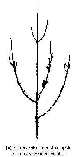
It is then possible to obtain an initial feedback on the collected data by displaying a 3D geometrical interpretation of a plant from the MTG. This notably allows the user to rapidly browse the overall database. For instance, a geometric interpretation of the 5th plant in the set of plants described in the MTG can be computed and plotted using the primitive PlantFrame as follows, ( Figure 3-7a):

geom_struct = PlantFrame(plant_list[4])
Plot(geom_struct)

Todo

continue to adapt the documenation from here including example here above

Such reconstructions can be carried out even if no geometric information is available in the collected data. In this case, algorithms are used to infer the missing data where possible (otherwise, default information is used) [19]. In other cases, plants are precisely digitised and the algorithms can provide accurate 3D geometric reconstructions [7] [22] [46] [48].

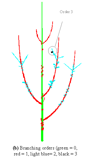
Apart from giving a natural view of the plants contained in the database, these 3D reconstructions play another important role: they can be used as a support to graphically visualise how various sorts of information are distributed in the plant architecture. Figure 3-7b for example shows the organisation of plant components according to their branching order (trunk components have order 0, branch components have order 1, etc.). This would be obtained by the following commands:

color_order(_x) = Switch Order(_x) Case 0: MediumGrey
    Case 1: DarkGrey Case 2: LightGrey Case 3: Black
    Default: White
Plot(geom_struct, Color=color_order)

This representation emphasises different informations related to the branching order: it can be seen in Figure 3-7b that the maximum branching order is 4, that this order is reached only once in the tree crown, and that this occurs at a floral site (black component).

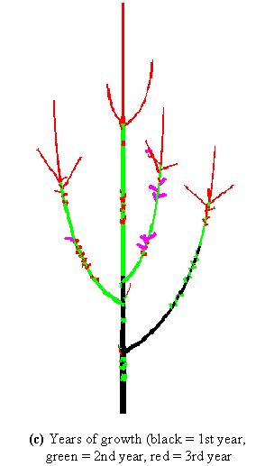
The use of the 3D representation of plant structure can also be illustrated in the context of plant growth analysis. The year in which each component grew can be retrieved from a careful analysis of the plant morphological makers. If this information is recorded in the MTG, it is then possible to colour the different components accordingly. Figure 3-7c shows, for instance, that a branch appeared on the trunk during the first year of growth. This information can then be linked to other data, e.g. the branching order of a component or the number of fruits borne by a component, and thus provides deeper insight into the plant growth process.

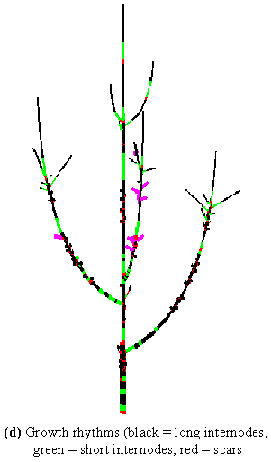
Thanks to the multiscale nature of the plant representation, more or less detailed information can be projected onto the plant structure. Let us consider again the context of plant growth analysis. Plant growth is characterised by rhythms that result in the production of long internodes during periods of high activity and short internodes during rest periods (indicated on the plant by scares close together). These informations, at the level of internodes, can be projected onto the plant 3D structure (Figure 3-7d). Like the year of growth, this information enables us to access plant growth dynamics, but now, at an intra-year scale.

Finally, another use for the virtual reconstruction of measured plants is illustrated in Figure 3-8a and 8b. These plants have been reconstructed from the MTG at the scale of each leafy internode. This enables us to obtain a natural representation of the plant which can be used for instance in models that are intended to describe the interaction of the plant and its environment (e.g. light) at a detailed level, e.g. [41]. More generally, the user can plot a set of plants from the database (Figure 3-9):

orchard = aml.PlantFrame(plant_list)
aml.Plot(orchard)

4.3. Extraction of data samples

Visualizing informations projected onto the 3D representation of plants is one way to explore the database. More quantitative explorations can be carried out and the most simple of these consists of studying how specific characters are distributed in the architecture of the plant population. To do this, samples of components are created corresponding to some topological or morphological criteria, and the distributions of one or several characters (target characters) are studied on this sample. This data extraction always follows the three following steps:

Firstly, a sample of components is created to study the target character. Secondly, the character itself is defined. It may be more or less directly derived from the data recorded in the field. For example, it is straightforward to define the diameter of a component if this has been measured in the field. On the other hand, the maximum branching order of the components that are borne by a given component needs some computation. Thirdly, the target character is computed for each component of the selected sample of components.

The output of these three operations is a set of values that can be analysed and visualised in various ways. Let us assume for instance that we wish to determine the distribution of the number of internodes produced during a specific growth period for all the plants in the database. It is first necessary to determine the sample of components on which we wish to study this distribution. In our case, we assume that we are interested in the growth units of the trunk that are produced during the first year of growth. This would be written as:

sample = Foreach _component In growth_unit_list:
    Select(_component,Order(_component) == 0 And
    Index(_component) == 90)

The variable sample thus contains the set of growth units whose order is 0 (i.e. which are parts of trunks) and whose growth year is 1990 (assuming 1990 corresponds to the first year of growth). The second step consists of defining the target character. This can be done by defining a corresponding function:

nb_of_internodes = lambda x: len(Components(x))

The number of internodes of a component _x (assumed to be a growth unit) is defined as the size of the set of components that compose this growth unit _x (assuming that growth units are composed of internodes). Finally, this function is applied to each component in the previously selected sample and the corresponding histogram is plotted (Figure 3-10):

sample_values = Histogram(Foreach _component In sample :nb_of_internodes(_component))
Plot(sample_values)

This example illustrates the kind of interaction a user may expect from the exploration of tree architecture. In the field, the growth units of the trunks produced during the first year of growth present a variable length, ranging roughly from 10 to 100 internodes. However, the quantitative exploration of the database shows that the histogram exhibits two relatively well-separated sub-populations of components (Figure 3-10). The sub-population of short components corresponds to the first annual shoots of the trunk, made up of two successive intra-annual growth units, while the sub-population of long components corresponds to the first annual shoots made up of a single growth unit.

In order to separate and characterise these two sub-populations, we can make the assumption that the global distribution is a mixture of two parametric distributions, more precisely, two negative binomial distributions. The parameters of this model can be estimated from the above histogram as follows:

mixture = Estimate(sample_value, "MIXTURE","NEGATIVE_BINOMIAL", "NEGATIVE_BINOMIAL")
Plot(mixture)

For all parametric models in the system, the function Estimate performs both parameter estimation and computation of various quantities (likelihood of the observed data for the estimated model, theoretical characteristics, etc) involved in the validation stage. As demonstrated by the cumulative distribution functions in Figure 3-11b, the data are well fitted by the estimated mixture of two negative binomial distributions. The weights of the two components of the mixture are very close (0.49 / 0.51), the first being centred on 21 internodes and the second on 53 internodes (Figure 3-11a). Due to the small overlap of these two mixture components (Figure 3-11a), the extracted sample can be optimally split up into two optimal sub-populations with a threshold fixed at 37.

As illustrated in this example, using AMAPmod, the user can query the database, make assumptions and look for data regularities. This interactive exploration process enables the user to build a rich and detailed mental representation of the architectural database, which relies on various complementary viewpoints.

4.4. Extraction and analysis of biological sequences

The previous section illustrates the extraction of a simple sample type, made up of numeric values. In this section, we consider a more complex sample type, made up of sequences of values. For example, in the apple tree database, let us consider sequences of lateral productions along trunks. Our aim is to analyse how lateral branches are distributed along the trunks of hybrids.

The sequences are coded as follows: for each plant, the 90 annual shoot of the trunk is described node by node from the base to the top. Each node is qualified by the type of lateral production (latent bud: 0, one-year-delayed short shoot: 1, one-year-delayed long shoot: 2 and immediate shoot: 3). This sample of sequences is built as follows:

AML> seq = Foreach _component In growth_unit_sample :
Foreach _node In Axis(_component, Scale -> 4) :
Switch lateral_type(_node)
Case BUD: 0 Case SHORT: 1 Case LONG: 2
Case IMMEDIATE: 3 Default: Undef

The AML variable growth_unit_sample contains the set of growth units of interest (assumed to be selected before). For each component in this set, the array of nodes that compose its main axis is browsed by the second Foreach construct. Finally, for each node, a function lateral_type() (defined elsewhere) is used to encode the nature of the lateral production at that node.

Figure 3-12 illustrates the diversity of annual shoot branching structures encountered in the studied hybrid family, which results from the different branching habits of the two parents. In our context, we wish to characterise and classify the hybrids according to their branching habits. The difficulty arises from the fact that the branching pattern is made of a succession of branching zones which are not characterised by a single type of lateral production but by a combination of types (e.g. short shoots interspersed with latent buds). We shall use this example to illustrate how parametric models may be used in AMAPmod to identify and characterize successive branching zones along these annual shoots.

We assume that sequences have a two-level structure, where annual shoots are made up of a succession of zones, each zone being characterised by a particular combination of lateral production types. To model this two-level structure, we use a hierarchical model with two levels of representation. At the first level, a semi-Markov chain (Markov chain with null self-transitions and explicit state occupancy distributions) represents the succession of zones along the annual shoots and the lengths of each zone [6] [28] [29]. Each zone is represented by a state of the Markov chain and the succession of zones are represented by transitions between states. The second level consists of attaching to each state of the semi-Markov chain a discrete distribution which represents the lateral productions types observed in the corresponding zone. The whole model is called a hidden semi-Markov chain [26] [27].

The model parameters are estimated from the extracted sample of sequences by the function Estimate:

hsmc = Estimate(seq, "HIDDEN_SEMI-MARKOV", initial_hsmc,Segmentation = True)

The first argument seq represents the extracted sequences, “HIDDEN_SEMI-MARKOV” specifies the family of models and initial_hsmc is an initial hidden semi-Markov chain which summarises the hypotheses made in the specification stage. An optimal segmentation of the sequences is required by the optional argument Segmentation set at True.

The hidden semi-Markov chain built from the 90 annual shoots of the 102 hybrids is depicted in Figure 3-13 with the following convention: each state is represented by a box numbered in the lower right corner. The possible transitions between states are represented by directed edges with the attached probabilities noted nearby. Transient states are surrounded by a single line while recurrent states are surrounded by a double line. State i is said to be recurrent if starting from state i, the first return to state i always occurs after a finite number of transitions. A nonrecurrent state is said to be transient. The state occupancy distributions which represent the length of the zones in terms of number of nodes are shown above the corresponding boxes. The possible lateral productions observed in each zone are indicated inside the boxes, the font sizes being roughly proportional to the observation probabilities(for state 3, these probabilities are 0.1, 0.62 and 0.28 while for state 4, these probabilities are 0.01, 0.07 and 0.92 for latent bud, one-year-delayed short shoot and one-year-delayed long shoot respectively). State 0 which is the only transient state is also the only initial state as indicated by the edge entering in state 0. State 0 represents the basal non-branched zone of the annual shoots. The remaining five states constitute a recurrent class which corresponds to the stationary phase of the sequences.

Building a parametric model gives us a global insight into the structure of the 90 annual shoot of the trunk for the 102 hybrids. The adequacy of the estimated model to the data is checked by examining the fitting of theoretical characteristic distributions computed from the model parameters to the corresponding observed characteristic distributions extracted from the data. Counting characteristic distributions for example focus on the number of occurrences of a given feature per sequence. The two features of interest are the number of series (or clumps) and the number of occurrences of a given lateral production type per sequence. The fits of counting distributions (Figure 3-14) can be plotted by the following function:

Plot(hsmc, "Counting")

In addition, the optimal segmentation of the observed sequences in successive zones (Figure 3-12) can be extracted from the model as a by-product of estimation of model parameters by the following function:

segmented_seq = ExtractData(hsmc)

segmented_seq represents the observed sequences augmented by a variable which contains the corresponding optimal state sequences (Figure 3-12). A careful examination of this optimal segmentation help us highlight a discriminating property: it suggests using the absence of state 4 in this optimal segmentation as a discrimination rule between hybrids closer to the Wijcik parent than to the Baujade parent (and conversely). State 4 corresponds to a dense long branching zone characteristic of the Baujade parent. Two sub-populations close to each of the parents are extracted by the function ValueSelect relying on the absence/presence of state 4 on the 1st variable:

wijcik_seq = ValueSelect(segmented_seq, 1, 4,Mode -> Reject)
baujade_seq = ValueSelect(segmented_seq, 1, 4,Mode -> Keep)

Simply counting the number of axillary long shoots per sequence would not have been sufficient, since for a given number of long shoots, these can be either scattered (Figure 3-12c) or aggregated in a dense zone (Figure 3-12d). This is confirmed by comparing the empirical distributions of the number of series with the number of occurrences of axillary long shoots per sequence extracted from the two hybrid sub-populations. The empirical distributions of the number of series/number of occurrences of axillary long shoots (coded by 2) per sequence for the sub-population close to the Wijcik parent can be simultaneously plotted by the following function (Figure 3-15a):

AML> Plot(ExtractHistogram(wijcik_seq, "NbSeries", 2, 2), ExtractHistogram(wijcik_seq, "NbOccurrences", 2, 2))

These empirical distributions are very similar for the sub-population close to the Wijcik parent, (Figure 3-15a). Most of the series are thus composed of a single long shoot. These empirical distributions are very different for the sub-population close to the Baujade parent, (Figure 3-15b). In this case, the series are frequently composed of several successive long shoots.

The studied sample of sequences encompasses a broad spectrum of branching habits ranging from the Wijcik to the Baujade parent one. Hence, the building of a parametric model is mainly used for identifying a discrimination rule to separate the initial sample of branching sequences into two sub-samples.

documentation status

Documentation adapted from the AMAPmod user manual version 1.8.

4.5. Bibliography

[1]

1998. Architecture et modélisation en arboriculture fruitière, Actes du 11ème colloque sur les recherches fruitières. INRA-Ctifl, Montpellier, France.

[2]

Barthélémy, D., 1991. Levels of organization and repetition phenomena in seed plants. Acta Biotheoretica, 39: 309-323.

[3]

Bouchon, J., de Reffye, P. et Barthélémy, D. (Eds), 1997. Modélisation et simulation de l’architecture des végétaux. Science Update. INRA Editions, Paris, France, 435 pp.

[4]

Caraglio, Y. et Dabadie, P., 1989. Le peuplier. Quelques aspects de son architecture. In: “ Architecture, structure, mécanique de l’arbre “ Premier séminaire interne, Montpellier (FRA) 01/89, pp. 94-107.

[5]

Cilas, C., Guédon, Y., Montagnon, C. et de Reffye, P., 1998. Analyse du suivi de croissance d’un cultivar de caférier (Coffea canephora Pierre) en Côte d’Ivoire. In: Architecture et modélisation en arboriculture fruitière, 11ème colloque sur les recherches fruitières, Montpellier, France 5-6/03/1998, INRA-Ctifl, pp. 45-55.

[6]

Costes, E. et Guedon, Y., 1997. Modelling the sylleptic branching on one-year-old trunks of apple cultivars. Journal of the American Society for Horticultural Science, 122(1): 53-62.

[7]

Costes, E., Sinoquet, H., Godin, C. et Kelner, J.J., 1999. 3D digitizing based on tree topology : application to study th variability of apple quality within the canopy. Acta Horticulturae, in press.

[8]

de Reffye, P., 1982. Modèle Mathématique aléatoire et simulation de la croissance et de l’architecture du caféier Robusta. 3ème Partie. Etude de la ramification sylleptique des rameaux primaires et de la ramification proleptique des rameaux secondaires. Café Cacao Thé, 26(2): 77-96.

[9]

de Reffye, P., Dinouard, P. et Barthélémy, D., 1991. Modélisation et simulation de l’architecture de l’Orme du Japon Zelkova serrata (Thunb.) Makino (Ulmaceae): la notion d’axe de référence. In: 2ème Colloque International sur l’Arbre, Montpellier (FRA) 9-14/09/90. Naturalia Monspeliensa, Vol. hors-série, pp. 251-266.

[10]

de Reffye, P., Edelin, C., Françon, J., Jaeger, M. et Puech, C., 1988. Plant models faithful to botanical structure and development. In: SIGGRAPH’88, Atlanta (USA) 1-15/08/88. C.G.S.C. Proceedings, Vol. 22, pp. 151-158.

[11]

de Reffye, P. et al., 1995. A model simulating above- and below- ground tree architecture with agroforestry applications. In: Agroforestry : Science; Policy and Practice, 20th IUFRO World Congress, F.L. Sinclair (Ed.), Tampere, Finlande 06-12/08/1995. Agroforestry Systems, Vol. 30, pp. 175-197.

[12]

Dempster, A.P., Laird, N.M. et Rubin, D.B., 1977. Maximum likelihood from incomplete data via the EM algorithm (with discussion). Journal of the Royal Statistical Society, Series B, 39: 1-38.

[13]

Ferraro, P. et Godin, C., 1998. Un algorithme de comparaison d’arborescences non ordonnées appliqué à la comparaison de la structure topologique des plantes. In: SFC’98, Recueil des Actes, Montpellier, France 21-23/09/1998, Agro Monpellier, pp. 77-81.

[14]

Ferraro, P. et Godin, C., 1999. A distance measure between plant architectures. Annales des Sciences Forestières: accepté.

[15]

Fisher, J.B. et Weeks, C.L., 1985. Tree architecture of Neea (Nyctaginaceae) : geometry and simulation of branches and the presence of two different models. Bulletin du Muséum National d’Histoire Naturelle, section B Adansonia, 7(4): 385-401.

[16]

Fitter, A.H., 1987. An architectural approach to the comparative ecology of plant root systems. New Phytologist, 106(Suppl.): 61-77.

[17]

Fournier, D., Guédon, Y. et Costes, E., 1998. A comparison of different fruiting shoots of peach trees. In: IVth International Peach Symposium, Bordeaux, France , Vol. 465(2), pp. 557-565.

[18]

Frijters, D. et Lindenmayer, A., 1976. Developmental descriptions of branching patterns with paraclidial relationships. In: Formal Languages, Automata and Development, G. Rozenberg et A. Lindenmayer (Eds), Noordwijkerhout, The Netherlands , North-Holland Publishing Company, pp. 57-73.

[19]

Godin, C., Bellouti, S. et Costes, E., 1996. Restitution virtuelle de plantes réelles : un nouvel outil pour l’aide à l’analyse de données botaniques et agronomiques. In: L’interface des mondes réels et virtuels, 5èmes Journées Internationales Informatiques, Montpellier, France 22-24/05/96, pp. 369-378.

[20]

Godin, C. et Caraglio, Y., 1998. A multiscale model of plant topological structures. Journal of Theoretical Biology, 191: 1-46.

[21]

Godin, C. et Costes, E., 1996. How to get representations of real plants in computers for exploring their botanical organisation. In: International Symposium on Modelling in Fruit Trees and Orchard Management, Avignon (FRA) 4-8/09/95, ISHS. Acta Horticulturae, Vol. 416, pp. 45-52.

[22]

Godin, C., Costes, E. et Caraglio, Y., 1997. Exploring plant topology structure with the AMAPmod software : an outline. Silva Fennica, 31(3): 355-366.

[23]

Godin, C., Costes, E. et Sinoquet, H., 1999. A method for describing plant architecture which integrates topology and geometry. Annals of Botany, 84(3): 343-357.

[24]

Godin, C., Guédon, Y. et Costes, E., 1999. Exploration of plant architecture databases with the AMAPmod software illustrated on an apple-tree bybird family. Agronomie, 19(3/4): 163-184.

[25]

Godin, C., Guédon, Y., Costes, E. et Caraglio, Y., 1997. Measuring and analyzing plants with the AMAPmod software. In: Plants to ecosystems - Advances in Computational Life Sciences 2nd International Symposium on Computer Challenges in Life Science. M.T. Michalewicz (Ed.). CISRO Australia, Melbourne, Australie, pp. 53-84.

[26]

Guédon, Y., 1998. Analyzing nonstationary discrete sequences using hidden semi- Markov chains. Document de travail du programme Modélisation des plantes, 5-98. CIRAD, Montpellier, France, 41 pp.

[27]

Guédon, Y., 1998. Hidden semi-Markov chains: a new tool for analyzing nonstationary discrete sequences. In: 2nd International Symposium on Semi-Markov models: theory and applications, J. Janssen et N. Limnios (Eds), Compiègne, France 09-11/12/1998, Université de Technologie de Compiègne, pp. 1-7.

[28]

Guédon, Y., Barthélémy, D. et Caraglio, Y., 1999. Analyzing spatial structures in forests tree architectures. In: Salamandra (Ed) Empirical and process-based models for forest tree and stand growth simulation, Oeiras, Portugal 21-27/09/1997, pp. 23-42.

[29]

Guédon, Y. et Costes, E., 1999. A statistical approach for analyszing sequences in fruit tree architecture. In: Wagenmakers P.S., van der Werf W., Blaise Ph. (Eds), 5th International Symposium on Computer modelling in fruit research and orchard management, Wageningen, The Netherlands 28-31/07/1998. Acta Horticulturae, pp. 271-280.

[30]

Hallé, F. et Oldeman, R.A.A., 1970. Essai sur l’architecture et la dynamique de croissance des arbres tropicaux. Monographie de Botanique et de Biologie Végétale, Vol. 6. Masson, Paris, 176 pp.

[31]

Hallé, F., Oldeman, R.A.A. et Tomlinson, P.B., 1978. Tropical trees and forests. An architectural analysis. Springer-Verlag, New-York.

[32]

Hanan, J. et Room, P., 1997. Practical aspects of plant research. In: Plants to ecosystems - Advances in Computational Life Sciences 2nd International Symposium on Computer Challenges in Life Science. M.T. Michalewicz (Ed.). CISRO Australia, Melbourne, Australie, pp. 28-43.

[33]

Harper, J.L., Rosen, B.R. et White, J., 1986. The growth and form of modular organisms. The Royal Society, London.

[34]

Honda, H., 1971. Description of the form of trees by the parameters of the tree-like body : Effects of the branching angle and the branch length on the shape of the tree-like body. Journal of Theoretical Biology, 31: 331-338.

[35]

Honda, H., Tommlinson, P. et Fisher, J.B., 1982. Two geometrical models of branching of tropical trees. Annals of Botany, 49: 1-12.

[36]

Jackson, J.E. et Palmer, J.W., 1981. Light distribution in discontinuous canopies: calculation of leaf areas and canopy volumes above defined irradiance contours for use in productivity modelling. Annals of Botany, 47: 561-565.

[37]

Jaeger, M. et de Reffye, P., 1992. Basic concepts of computer simulation of plant growth. In: The 1990 Mahabaleshwar Seminar on Modern Biology, Mahabaleshwar (IND) . Journal of Biosciences, Vol. 17, pp. 275-291.

[38]

Mitchell, K.J., 1975. Dynamics and simulated yield of Douglas-fir. Forest Science, 21(4): 1-39.

[39]

Prusinkiewicz, P. et Lindenmayer, A., 1990. The algorithmic beauty of plants. Springer Verlag.

[40]

Prusinkiewicz, P.W., Remphrey, W.R., Davidson, C.G. et Hammel, M.S., 1994. Modeling the architecture of expanding Fraxinus pennsylvanica shoots unsing L-systems. Canadian Journal of Botany, 72: 701-714.

[41]

Rapidel, B., 1995. Etude expérimentale et simulation des transferts hydriques dans les plantes individuelles. Application au caféier (Coffea arabica L.). Thèse Doctorat, Université des Sciences et Techniques du Languedoc (USTL), Montpellier, France, 246 pp.

[42]

Remphrey, W.R., Neal, B.R. et Steeves, T.A., 1983. The morphology and growth of Arctostaphylos uva-ursi (bearberry): an architectural model simulated colonizing growth. Canadian Journal of Botany, 61: 2451-2458.

[43]

Room, P. et Hanan, J., 1996. Virtual plants: new perspectives for ecologists, pathologists and agricultural scientists. Trends in Plant Science Update, 1(1): 33-38.

[44]

Ross, J.K., 1981. The radiation regim and the architecture of plant stands. Junk W. Pubs., The Hague, The Netherlands.

[45]

Sabatier, S., Ducousso, I., Guédon, Y., Barthélémy, D. et Germain, E., 1998. Structure de scions d’un an de Noyer commun, Juglans regia L., variété Lara greffés sur trois porte-greffe (Juglans nigra, J. regia, J. nigra x J. regia). In: Architecture et modélisation en arboriculture fruitière, 11ème colloque sur les recherches fruitières, Montpellier, France 5-6/03/1998, INRA-Ctifl, pp. 75-84.

[46]

Sinoquet, H., Adam, B., Rivet, P. et Godin, C., 1998. Interactions between light and plant architecture in an agroforestry walnut tree. Agroforestry Forum, 8(2): 37-40.

[47]

Sinoquet, H., Godin, C. et Costes, E., 1998. Mesure de l’architecture par digitalisation 3D. In: Numérisation 3D, Design et digitalisation, Création industrielle et artistique, Actes du Congrès, Paris, France 27-28/05/1998.

[48]

Sinoquet, H., Rivet, P. et Godin, C., 1997. Assessment of the three-dimensional architecture of walnut trees using digitising. Silva Fennica, 31(3): 265-273.

[49]

Sinoquet, H., Thanisawanyangkura, S., Mabrouk, H. et Kasemsap, P., 1998. Characterisation of the light environment in canopies using 3D digitising and image processing. Annals of Botany, 82: 203-212.

[50]

Zhang, K., 1993. A new editing based distance between unordered labeled trees. In: Combinatorial Pattern Matching CPM 93, 4th Annual Symposium, Padova, Italie 2-4/06/1993.